Analytical techniques can be used to solve some diffusion problems. However, the solutions obtained by analytical methods are not always suitable for computing numerical values of the solution in cases where the geometry is complex and the material properties are not uniform. Also, in many cases the analytical solutions do not apply (e.g. the boundary conditions will not permit a separation of variables) for solving the problem. In such cases, the analytical solution can be used to describe some of the fundamental characteristics of the solution being studied but the problem is solved again by numerical methods for the purpose of generating an accurate solution. With today's high-speed computers, numerical techniques are important for this type of problem.
The current density diffusion equation can be formulated as a boundary and initial value problem as
n0—2J = s ?J/?t
s.t. J(r, t) = 0 for t<0
?J(0, t)/?r = 0
J(r, 0) = dR(r)
dR(r) = 0 for 0=r<R and the following relation holds
? dR(r) dS = I0 for t=0 (dR is similar to a Dirac delta function)
and ? J dS = I(t) for t=0. Unfortunately, the above formulation is obtained after solving the above equation using analytical methods.
It is easy to set up the above equations in terms of a finite difference formulation. However, this approach does not allow us to specify the boundary conditions so that its solution can be obtained without starting off using the analytical solution. This fact is easily seen by looking at the analytical solution as t -> 0+. At t=0, the analytical solution for the step current input predicts that all the current passes on the outer surface (skin) of the conductor. This situation is impossible to model numerically. What can be done is that we will look at the analytical solution at some time t0+Dt and start off our numerical procedure by using the values of J(r, t0+Dt) as an initial condition.
This approach is messy and leads to computational difficulties in getting the solution started. For example, the outermost element of the conductor is assigned a value which probably would result in the discrepency that the integral of the current density through the cross section of the conductor might not add up to be the total current in the conductor and thus all the values of the current density would be scaled accordingly. We will not use this approach and will reformulate our problem in another way, working directly with the magnetic vector potential.
On the basis of the mathematical model described by equations (2.30) and (2.31), we can develop, using finite difference or finite element methods, an algorithm for the numerical calculation of Az(r, q, t).
As we have stated in equations (30) and (31) above, we want to solve the system :
(4.1) n0 —2 A - s ?A/?t = - Js = - s C(t)
(4.2) s C(t) - s ?A/?t = JT
where
C(t) = - — f gradient of the scaler electric potential
defined over the surface of the conductor
at time tn
Js = -s — f the source current density in the conductor
-s ?A/?t the eddy current density in the conductor
JT the total current density in the conductor
s the conductivity of the conductor
n0 the reluctivity of free space,
in our case a constant
This formulation is discussed in Garg and Weiss [4.1]. If we integrate this above equation over the cross-section F of the conductor, we obtain our current constraint
(4.3) ?F s C(t) dS - ?F s ?A/?t dS = I(t)
where I(t) is the given current in the conductor at time t. Because the conductor is uniform in the z-direction, we have that — f is a constant over the surface of the conductor:
(4.4) C(t) ?F s dS - ?F s ?A/?t dS = I(t)
Solving this equation (4.4) for C(t) and substituting into equation (4.1) yields
?F s ?A/?t dS I(t)
(4.5) n0 —2 A - s ?A/?t = - ——————————— - ————————
?F s dS ?F s dS
The problem to which we will apply the finite difference methods describes an infinitely long cylindrical conductor having a radius R. This conductor will be placed in free space and carry a current I(t) with a coaxial return at infinity. Inside the conductor, the conductivity will be that of copper at 273 degrees Kelvin, and outside the conductor it will be that of free space, namely zero.
In cylindrical coordinates, the Laplacian is
(4.5b) —2A = ?2A/?r2 + 1/r ?A/?r + 1/r2 ?2A/?q2
where r is the radial distance. With radial symmetry (?A/?q = 0), this
reduces to
(4.5c) —2A = ?2A/?r2 + 1/r ?A/?r .
In our problem F is a disc of radius R. Now a grid for the cross-section is defined by concentric circles at rk = k (?r), 0<k=M, where Dr = R/M, and the radial lines qj = j (?q) where Dr and Dq are fixed for the mesh of the problem, see Smith [4.2] or Lapidus and Pinder [4.3]. The radial symmetry shows that the solution is independant of q. We will work with a two-dimensional mesh using one direction to denote time and the other direction to denote the radial distance. The mesh in time has equally spaced nodes at tn= t0 + n Dt. The symbol a(k, n) denotes the finite difference approximation to the magnetic vector potential at the radial node rk at time tn. Our interpolation formula in time requires only the nodes at the previous time and the current time. Thus the problem is further simplified by using only a two-tier grid. This is illustrated below.
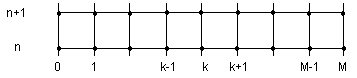
Fig. 4.1 The mesh for the problem. We apply the method of finite differences to this problem using small increments ?r and ?t. The solution we obtain will be an approximation to the true solution because of this finite increment. The finite difference approximations given in angle independent polar coordinates are obtained from Taylor's formula with a remainder term and are, see Vermuri and Karplus[4.4] or Vichnevetsky [4.5]
?A a(k, n+1) - a(k, n)
(4.6a) ––– (rk, tn) = –––––––––––––––––– + C ?t,
?t Dt
C = (1/2!) ?2A(k, n+lDt)/?2t, 0 < l < 1
?2A(rk,tn) a(k+1, n) - 2 a(k, n) + a(k-1, n)
(4.6b) —————— = ————————————————————— + K(?r)2 ?r2 ?r . ?r
1 a(k+1, n) - a(k-1, n)
+ ——— —————————————— + K' ?r
rk 2 ?r
K = (1/3!) ?3A(k+m Dr, n)/?r3, 0 < m < 1
K = (1/2!) ?2A(k+m Dr, n)/?r2, -1 < m' < 1
where an equally-spaced grid is used to avoid programming complicated formulas and algorithms. To do the integration, we use the midpoint rule
M
? A dS = ? a(k, n) Fk Dr + O(Dr2)
F k = 0
where
a(k, n) the magnetic vector potential at node k and
at time tn
s(k, n) the conductivity at node l and at time tn
Fk area per unit radial distance of the element, Fk=2prk
k nodal point at the center of the element;
indexing begins with 0 and ends with M
M maximal index on the region accounted for by the
conductor
n index on time, values are all known for time tn,
unknown values correspond to time tn+1
tn to + ?t * n, for equally spaced time nodes
to initial time, in our case to = 0
?t increment in time, usually the same for all t
?r increment in radial distance
The reason for using the midpoint rule is that the values are only specified at our nodal point (which is the center of our finite difference element) and that the approximation is O(Dr2).
A great deal of work has been done on the homogeneous diffusion equation (without the source term):
?2A/?r2 + 1/r ?A/?r = s/n0 ?A/?t.
In this case, the computation is straight forward. However, since the equation relates finite quantities in different directions, namely along the radius and along the direction of time, a question arises involving the decision for which nodes the scheme should be implemented. We have a time marching problem in that we obtain all the values at a fixed time before we can go on to calculate the values at the next time step.
One choice is to approximate all our quantities relative to the node (k, n). In this case, we have the Euler explicit approximation:
a(k+1, n) -2a(k, n) + a(k-1, n) = 1/q[a(k, n+1) - a(k, n)].
where q = n0 Dt/ s Dr2. Another choice is to approximate relative to the node
(k, n+1). This is called the Euler backward or Larson (implicit) approximation:
a(k+1, n+1) -2a(k, n+1) + a(k-1, n+1) = 1/q[a(k, n+1) - a(k, n)].
Each of these schemes is biased toward the node at which the space derivative is matched to the time derivative. One improvement is to use an average of the second derivatives at the nodes (k, n) and (k, n+1) and to center the approximation relative to this. This is called the Crank-Nicolson approximation, see Twizell [4.6].
1/2 [a(k+1, n) -2a(k, n) + a(k-1, n)]
+ 1/2[a(k+1, n+1) -2a(k, n+1) + a(k-1, n+1)]
= 1/q[a(k, n) - a(k, n-1)].
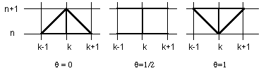
Figure 4.2 Computational molecule for the homogeneous diffusion equation.
For the homogeneous diffusion equation, the Euler explicit method is used because it allows the direct calculation of the values at the next time step without solving a tridiagonal system of many equations. The truncation error is of the form E1 = K1 Dr2 + K'1 Dr + C1 Dt (see Evans[4.7]), for q =1/2 where
q = n0 Dt/s Dr2 , C1 = (1/2!) ?2A(k, n+l1 Dt)/?2t, 0 < l1 < 1,
K1 = (1/3!) ?3A(k+m1 Dr, n)/?r3, 0 < m1 < 1,
K'1 = (1/2!) ?2A(k+m1 Dr, n)/?r2, -1 < m'1 < 1. For q > 1/2, this formulation is unstable. By using the values at the previous time in the adjacent nodes in modeling the diffusion, the explicit scheme introduces characteristics into the behavior in that information at the jth node takes a time kDt to arrive at j+kth node. Implementation of an algorithm in which the time step is too large in relation to the space nodes results in instability. For the differential form of the diffusion equation and for the physical problem, the diffusion effects still occur at this same rate but the transfer of information is instantaneous (is that of the speed of light). The presence of our source term and the coupling to the current constraint do not permit us to solve the system by merely taking a combination of values of surrounding nodes from the previous time step.
The Crank-Nicolson method has been the preferred method for the solution of the parabolic partial differential equations in one space dimension. Its advantage is higher precision for a given step size. The error term is of the form E2 = K2 Dr2 + K'2 2Dr + C2 Dt2, where C2 = (1/2!) ?3A(k, n+l2 Dt)/?3t, 0 < l2 < 1,
K2 = (1/3!) ?3A(k+m2 Dr, n)/?r3, 0 < m2 < 1,
K'2 = (1/2!) ?2A(k+m'2 Dr, n)/?r2, -1 < m'2 < 1. It also retains the parabolic character of the original equation because the solution at the point xj at time tn+1 is influenced not only by all the earlier values, but also by the solution at all other points at time tn+1 as well. The disadvantage is the need to solve a tri-diagonal matrix system at each time step. However, this is a straight forward procedure.
The Larson totally implicit method has also been used to solve parabolic systems. The truncation error is of the form E3 = K3 Dr2 + K'3 2Dr + C3 Dt, where C3 = (1/2!) ?2A(k, n+l3 Dt)/?2t, 0 < l3 < 1,
K3 = (1/3!) ?3A(k+m3 Dr, n)/?r3, 0 < m3 < 1,
K'3 = (1/2!) ?2A(k+m'3 Dr, n)/?r2, -1 < m'3 < 1 . This scheme is of the same order as is the explicit scheme but one order lower in time than is the Crank Nicolson formulation at the same computational cost. Usually, C3 << C1. However, it should be pointed out that it is not only the magnitude of the order which is important, but also the constant Ki. One should be aware of the possibility that for a certain range of the parameters, ?t and ?r, the lower order method may be more accurate because the constant C3 may be less than C2 Dt. In essence, this may be trivial since it is very costly to calculate the constants Ci and Ki because of their dependance on so many parameters which occur in the geometry of each problem. When modelling our problem using relatively large time steps (that is for q ª10), we avoid using the Crank-Nicolson scheme because of the oscillatory behavior exhibited even though it is stable. Zienkiewicz and Morgan [4.8] illustrate this. However, the most important reason we use the totally implicit method is for the advantages that occur in the special form of the forcing term. More will be stated about this in the section on finite elements.
Now we would like to write our difference equation using a weighted average approximation. Considering the different cases - for q = 0, this is a Euler explicit forward difference formulation, for q=1/2, this is a Crank-Nicolson implicit central difference formulation, and for q=1, this is a fully implicit backward difference formulation. The differential equation (4.5) becomes the difference equation
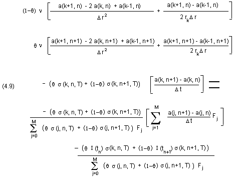
where
a(k, n) is the magnetic vector potential at the
kth node in space and nth node in time,
Fk the area of the region center at the node k,
s(k, n, T) the conductivity of the region centered at the node at a temperature T,
I(tn) the current magnitude at time tn
?t time step,
?r space increment,
q variable weight parameter, 0=q=1
k=0 node corresponding to the center of the conductor,
k=M node corresponding to the outer-most region
of the conductor,
n=0 node corresponding to the initial time,
n=N node corresponding to the final time,
.
This equation as it stands has as unknowns s(k, n+1, T) and a(k, n+1). The coefficients s(k, n+1, T) can be estimated using s(k, n, T) and extrapolating the anticipated temperature rise. However, since this effect is negligible over one time step, we set s(k, n+1, Tn) = s(k, n, Tn) and update the value at the end of the time step.
We make one more assumption - the reluctivity, n, is a constant since the material is non-ferromagnetic. If this were not so, we would have to specify its behavior.
The boundary conditions for this problem are also straight forward.
At the Neumann boundary we have ?A/?r = 0. At r=0, we should use the condition that a(-1, n) = a(1, n). Hence in our finite differences, at k = 0, we must change the coding so that we do not address variables out of bounds. Also, we must change the form of the difference equation (4.6b) because of an apparent singularity of 1/r at the origin. This problem exists only because of the choice of the cylindrical coordinate system. If we take the limit as r tends to zero of equation (4.5c), we get by application of l'Hospital`s rule
(4.11) —2A (r=0) = limit ?2A/?r2 + 1/r ?A/?r = 2 ?2A/?r2 .
r -> 0
At the center of our grid, we change the computation molecule to use the above information.
Notice that since s=0 in free space, our differential equation (4.5) reduces to Laplace's equation in this region. At the Dirichlet boundary, we have A equal to some prescribed value. We will not be trying to couple our finite difference method to the solution which holds outside the conductor, namely
A(r, t) = -moI(t)/2p ln(r) + K, r > R (see equation 2.65) where K is an arbitrary constant. We choose to end our finite difference mesh at r=R, where R is the radius of the conductor. A(r, t) is a potential and, thus, it can be specified up to a constant. Since we have radial symmetry, we might as well make it zero at the end our mesh. Moreover, we are interested only in the change in A in time so that its absolute value is irrelevant.
Through the use of Neumann's Fourier stability analysis, the above formulation is shown to be unconditionally stable when the source term is neglected, see Kreiss[4.9] and Khalig and Twizell [4.10]. We tried to show that this is also true when the source term is included, however the algebra becomes intractable and it is no longer possible to group the terms as was done for the simpler problem.
Conclusion
A method of calculating the eddy currents in a cylindrical conductor by a suddenly applied current to the system is given.
It is shown that the analysis of the eddy currents in a cylindrical transients current carrying conductor leads to the well known parabolic differential equation with given initial and boundary conditions. However, its application to eddy current distribution in the above cylinder after applying a current ramp input function as well as the study of the error in the presence of the source current density term were not previously done.
We illustrate the numerical techniques described in this section by presenting the results of numerical calculations where these techniques have been used to simulate the magnetic vector potential and the current density distribution modeled by equation (4.1) and (4.3) for several different times.
The plots of the magnetic vector potential a(r, t) and the current density vector J(r, t) and da(r, t)/dt are shown in figures 4.3, 4.4, and 4.5 . They indicate the changes of the above field quantities in an infinitely long circular cylindrical conductor as a function of its radius at four different times t=0.5 msec, 1.0 msec., 1.5 msec., and 2.0 msec. The magnetic vector potential is given in units of Volt seconds / meter. The current density is given in Amps/meter2.
Figure 4.3 Current density distribution vs. radial distance at four different times.
Figure 4.4 Magnetic vector potential distribution vs. radial distance at four different times.
Figure 4.5 The change in the magnetic vector potential distribution in time vs. radial distance at four different times.
Figure 4.6. Finite difference results at time = 1.0 msec, 2.0 msec, ..., 10.0 msec, using Dt = 0.25 msec. and constant conductivity, s = 5.0 x 10⁸.
Figure 4.7 Close-up of previous diagram.
References:
[4.1] Garg, V. K. and Weiss, J., "Finite element solution of Transient Eddy-Current Problems in Multiply-Excited Magnetic Systems," IEEE Transactions on Magnetics, September 1986, Vol. MAG-22, No. 5, pp. 1257-1259.
[4.2] Smith, G. D., Numerical Solution of Partial Differential Equations, Finite Difference Methods, Oxford University Press, 1978.
[4.3] Lapidus, L. and Pinder, G. F., Numerical Solution of Partial Differential Equations in Science and Engineering, John Wiley and Sons, New York, (1982)
[4.4] Vermuri, V. and Karplus, W. J., Digital Computer Treatment of Partial Differential Equations. Prentice - Hall, Inc., Englewood Cliffs, New Jersey (1981).
[4.5] Vichnevetsky, R. , Computer Methods for Partial Differential Equations, Vol. I, Prentice - Hall, Inc, (1981)
[4.6] Twizell, E. H., Computational Methods for Partial Differential Equations. Ellis Horwood Ltd. - John Wiley and Sons, New York (1984).
[4.7] Evans, A., Lecture Notes For Numerical Solutions to Differential Equations, McGill University, Spring 1985.
[4.8] Zienkiewicz and Morgan, Finite Elements and Approximations, John Wiley and Sons, (1983)
[4.9] Kreiss, H. O. , Numerical Methods for Solving Time Dependent Problems for Partial Differential Equations. Les Presses de L'Universite de Montreal, C. P. 6128, Succ. "A", Montreal, (1978)
[4.10] Khalig, A. Q. M. and Twizell, E. H., "L0-Stable Splitting Methods for the Simple Heat Equation in Two Space Dimensions with Homogeneous Boundary Conditions," SIAM Journal Numerical Analysis. Vol. 23, No. 3 June 1986, pp.473-484.